May 20, 2020

|
|
From my first year i always wanted to get selected for Gsoc and do some exiciting projects, but never took it seriously. When i reached my third year i made up my mind that it is a high time for preparig for Gsoc. For Gsoc 2020 i choose to apply to Sympy as i found this community very intresting. I took a head start and started contributing for four months before the application period. It was a really nice experience and i meet some really interesting people. I am glad that i made the right decision of choosing this organization.
May 17, 2020

|
|
This is the first official blog associated with GSoC 2020. I will be sharing the experience of the Community Bonding Period and work during this period after selection.
May 07, 2020

|
|


The results of Google Summer of Code were out on 04 May 2020 and I am pleased to share with you that my proposal with Sympy was accepted.
I would like to thank all the members of the organisation especially Kalevi Suominen for guiding me in my proposal and PR’s. I am really excited to work for such an amazing organization.
I will be working on my project, Amendments to Limit Evaluation and Series Expansion, during a period of 3 months spanning from June to August, under the mentorship of Kalevi Suominen and Sartaj Singh.
My primary focus will be to work on the series module and make it more robust as it is the backbone of all the limit evaluations performed by the library.
Looking forward for a really productive and wonderful summer ahead.
May 06, 2020
Name: Smit Lunagariya
May 05, 2020
|
|
|
I will be sharing my Pre-GSoC journey in this blog. I started exploring about the GSoC program around November 2019 and was quite interested in the open source. I began to look for the organisations and came across a Math and Physics library in python, SymPy.
March 31, 2020

|
|
Like most people, I've had a lot of free time recently, and I've spent some of it watching various YouTube videos about the Riemann Hypothesis. I've collected the videos I've watched into YouTube playlist. The playlist is sorted with the most mathematically approachable videos first, so even if you haven't studied complex analysis before, you can watch the first few. If you have studied complex analysis, all the videos will be within your reach (none of them are highly technical with proofs). Each video contains parts that aren't in any of the other videos, so you will get something out of watching each of them.
One of the videos near the end of the playlist is a lecture by Keith Conrad. In it, he mentioned a method by which one could go about verifying the Riemann Hypothesis with a computer. I wanted to see if I could do this with SymPy and mpmath. It turns out you can.
Background Mathematics
Euler's Product Formula
Before we get to the computations, let's go over some mathematical background. As you may know, the Riemann Hypothesis is one of the 7 Millennium Prize Problems outlined by the Clay Mathematics Institute in 2000. The problems have gained some fame because each problem comes with a $1,000,000 prize if solved. One problem, the Poincaré conjecture, has already been solved (Grigori Perelman who solved it turned down the 1 million dollar prize). The remainder remain unsolved.
The Riemann Hypothesis is one of the most famous of these problems. The reason for this is that the problem is central many open questions in number theory. There are hundreds of theorems which are only known to be true contingent on the Riemann Hypothesis, meaning that if the Riemann Hypothesis were proven, immediately hundreds of theorems would be proven as well. Also, unlike some other Millennium Prize problems, like P=NP, the Riemann Hypothesis is almost universally believed to be true by mathematicians. So it's not a question of whether or not it is true, just one of how to actually prove it. The problem has been open for over 160 years, and while many advances have been made, no one has yet come up with a proof of it (crackpot proofs aside).
To understand the statement of the hypothesis, we must first define the zeta function. Let
$$\zeta(s) = \sum_{n=1}^\infty \frac{1}{n^s}$$
(that squiggle $\zeta$ is the lowercase Greek letter zeta). This expression makes sense if $s$ is an integer greater than or equal to 2, $s=2, 3, 4, \ldots$, since we know from simple arguments from calculus that the summation converges in those cases (it isn't important for us what those values are, only that the summation converges). The story begins with Euler, who in 1740 considered the following infinite product:
$$\prod_{\text{$p$ prime}}\frac{1}{1 - \frac{1}{p^s}}.$$
The product ranges over all prime numbers, i.e., it is $$\left(\frac{1}{1 - \frac{1}{2^s}}\right)\cdot\left(\frac{1}{1 - \frac{1}{3^s}}\right)\cdot\left(\frac{1}{1 - \frac{1}{5^s}}\right)\cdots.$$ The fraction $\frac{1}{1 - \frac{1}{p}}$ may seem odd at first, but consider the famous geometric series formula, $$\sum_{k=0}^\infty r^k = \frac{1}{1 - r},$$ which is true for $|r| < 1$. Our fraction is exactly of this form, with $r = \frac{1}{p^s}$. So substituting, we have
$$\prod_{\text{$p$ prime}}\frac{1}{1 - \frac{1}{p^s}} = \prod_{\text{$p$ prime}}\sum_{k=0}^\infty \left(\frac{1}{p^s}\right)^k = \prod_{\text{$p$ prime}}\sum_{k=0}^\infty \left(\frac{1}{p^k}\right)^s.$$
Let's take a closer look at what this is. It is
$$\left(\frac{1}{p_1^s} + \frac{1}{p_1^{2s}} + \frac{1}{p_1^{3s}} + \cdots\right)\cdot\left(\frac{1}{p_2^s} + \frac{1}{p_2^{2s}} + \frac{1}{p_2^{3s}} + \cdots\right)\cdot\left(\frac{1}{p_3^s} + \frac{1}{p_3^{2s}} + \frac{1}{p_3^{3s}} + \cdots\right)\cdots,$$
where $p_1$ is the first prime, $p_2$ is the second prime, and so on. Now think about how to expand finite products of finite sums, for instance, $$(x_1 + x_2 + x_3)(y_1 + y_2 + y_3)(z_1 + z_2 + z_3).$$ To expand the above, you would take a sum of every combination where you pick one $x$ term, one $y$ term, and one $z$ term, giving
$$x_1y_1z_1 + x_1y_1z_2 + \cdots + x_2y_1z_3 + \cdots + x_3y_2z_1 + \cdots + x_3y_3z_3.$$
So to expand the infinite product, we do the same thing. We take every combination of picking $1/p_i^{ks}$, with one $k$ for each $i$. If we pick infinitely many non-$1$ powers, the product will be zero, so we only need to consider terms where there are finitely many primes. The resulting sum will be something like
$$\frac{1}{1^s} + \frac{1}{p_1^s} + \frac{1}{p_2^s} + \frac{1}{\left(p_1^2\right)^s} + \frac{1}{p_3^s} + \frac{1}{\left(p_1p_2\right)^s} + \cdots,$$
where each prime power combination is picked exactly once. However, we know by the Fundamental Theorem of Arithmetic that when you take all combinations of products of primes that you get each positive integer exactly once. So the above sum is just
$$\frac{1}{1^s} + \frac{1}{2^s} + \frac{1}{3^s} + \cdots,$$ which is just $\zeta(s)$ as we defined it above.
In other words,
$$\zeta(s) = \sum_{n=1}^\infty \frac{1}{n^s} = \prod_{\text{$p$ prime}}\frac{1}{1 - \frac{1}{p^s}},$$ for $s = 2, 3, 4, \ldots$. This is known as Euler's product formula for the zeta function. Euler's product formula gives us our first clue as to why the zeta function can give us insights into prime numbers.
Analytic Continuation
In 1859, Bernhard Riemann wrote a short 9 page paper on number theory and the zeta function. It was the only paper Riemann ever wrote on the subject of number theory, but it is undoubtedly one of the most important papers every written on the subject.
In the paper, Riemann considered that the zeta function summation,
$$\zeta(s) = \sum_{n=1}^\infty \frac{1}{n^s},$$
makes sense not just for integers $s = 2, 3, 4, \ldots$, but for any real number $s > 1$ (if $s = 1$, the summation is the harmonic series, which famously diverges). In fact, it is not hard to see that for complex $s$, the summation makes sense so long as $\mathrm{Re}(s) > 1$ (for more about what it even means for $s$ to be complex in that formula, and the basic ideas of analytic continuation, I recommend 3Blue1Brown's video from my YouTube playlist).
Riemann wanted to extend this function to the entire complex plane, not just $\mathrm{Re}(s) > 1$. The process of doing this is called analytic continuation. The theory of complex analysis tells us that if we can find an extension of $\zeta(s)$ to the whole complex plan that remains differentiable, then that extension is unique, and we can reasonably say that that is the definition of the function everywhere.
Riemann used the following approach. Consider what we might call the "completed zeta function"
$$Z(s) = \pi^{-\frac{s}{2}}\Gamma\left(\frac{s}{2}\right)\zeta(s).$$
Using Fourier analysis, Riemann gave a formula for $Z(s)$ that is defined everywhere, allowing us to use it to define $\zeta(s)$ to the left of 1. I won't repeat Riemann's formula for $Z(s)$ as the exact formula isn't important, but from it one could also see
-
$Z(s)$ is defined everywhere in the complex plane, except for simple poles at 0 and 1.
-
$Z(s) = Z(1 - s).$ This means if we have a value for $s$ that is right of the line $\mathrm{Re}(z) = \frac{1}{2},$ we can get a value to the left of it by reflecting it over the real-axis and the line at $\frac{1}{2}$ (to see this, note that the average of $s$ and $1 - s$ is $1/2$, so the midpoint of a line connecting the two should always go through the point $1/2$).

(Reflection of $s$ and $1 - s$. Created with Geogebra)
Zeros
Looking at $Z(s)$, it is a product of three parts. So the zeros and poles of $Z(s)$ correspond to the zeros and poles of these parts, unless they cancel. $\pi^{-\frac{s}{2}}$ is the easiest: it has no zeros and no poles. The second part is the gamma function. $\Gamma(z)$ has no zeros and has simple poles at nonpositive integers $z=0, -1, -2, \ldots$.
So taking this, along with the fact that $Z(s)$ is entire except for simple poles at 0 and 1, we get from $$\zeta(s) = \frac{Z(s)}{\pi^{-\frac{s}{2}}\Gamma\left(\frac{s}{2}\right)}$$
- $Z(s)$ has a simple pole at 1, which means that $\zeta(s)$ does as well. This is not surprising, since we already know the summation formula from above diverges as $s$ approaches 1.
- $Z(s)$ has a simple pole at 0. Since $\Gamma\left(\frac{s}{2}\right)$ also has a simple pole at 0, they must cancel and $\zeta(s)$ must have neither a zero nor a pole at 0 (in fact, $\zeta(0) = -1/2$).
- Since $\Gamma\left(\frac{s}{2}\right)$ has no zeros, there are no further poles of $\zeta(s)$. Thus, $\zeta(s)$ is entire everywhere except for a simple pole at $s=1$.
- $\Gamma\left(\frac{s}{2}\right)$ has poles at the remaining negative even integers. Since $Z(s)$ has no poles there, these must correspond to zeros of $\zeta(s)$. These are the so-called "trivial" zeros of the zeta function, at $s=-2, -4, -6, \ldots$. The term "trivial" here is a relative one. They are trivial to see from the above formula, whereas other zeros of $\zeta(s)$ are much harder to find.
- $\zeta(s) \neq 0$ if $\mathrm{Re}(s) > 1$. One way to see this is from the Euler product formula. Since each term in the product is not zero, the function itself cannot be zero (this is a bit hand-wavy, but it can be made rigorous). This implies that $Z(s) \neq 0$ in this region as well. We can reflect $\mathrm{Re}(s) > 1$ over the line at $\frac{1}{2}$ by considering $\zeta(1 - s)$. Using the above formula and the fact that $Z(s) = Z(1 - s)$, we see that $\zeta(s)$ cannot be zero for $\mathrm{Re}(s) < 0$ either, with the exception of the aforementioned trivial zeros at $s=-2, -4, -6, \ldots$.
Thus, any non-trivial zeros of $\zeta(s)$ must have real part between 0 and 1. This is the so-called "critical strip". Riemann hypothesized that these zeros are not only between 0 and 1, but are in fact on the line dividing the strip at real part equal to $1/2$. This line is called the "critical line". This is Riemann's famous hypothesis: that all the non-trivial zeros of $\zeta(s)$ have real part equal to $1/2$.
Computational Verification
Whenever you have a mathematical hypothesis, it is good to check if it is true numerically. Riemann himself used some methods (not the same ones we use here) to numerically estimate the first few non-trivial zeros of $\zeta(s)$, and found that they lied on the critical line, hence the motivation for his hypothesis. Here is an English translation of his original paper if you are interested.
If we verified that all the zeros in the critical strip from, say, $\mathrm{Im}(s) = 0$ to $\mathrm{Im}(s) = N$ are in fact on the critical line for some large $N$, then it would give evidence that the Riemann Hypothesis is true. However, to be sure, this would not constitute a proof. Hardy showed in 1914 that $\zeta(s)$ has infinitely many zeros on the critical strip, so only finding finitely many of them would not suffice as a proof. (Although if we were to find a counter-example, a zero not on the critical line, that WOULD constitute a proof that the Hypothesis is false. However, there are strong reasons to believe that the hypothesis is not false, so this would be unlikely to happen.)
How would we verify that the zeros are all on the line $1/2$. We can find zeros of $\zeta(s)$ numerically, but how would we know if the real part is really exactly 0.5 and not 0.500000000000000000000000000000000001? And more importantly, just because we find some zeros, it doesn't mean that we have all of them. Maybe we can find a bunch of zeros on the critical line, but how would we be sure that there aren't other zeros lurking around elsewhere on the critical strip?
We want to find rigorous answers to these two questions:
-
How can we count the number of zeros between $\mathrm{Im}(s) = 0$ and $\mathrm{Im}(s) = N$ of $\zeta(s)$?
-
How can we verify that all those zeros lie on the critical line, that is, they have real part equal to exactly $1/2$?
Counting Zeros Part 1
To answer the first question, we can make use of a powerful theorem from complex analysis called the argument principle. The argument principle says that if $f$ is a meromorphic function on some closed contour $C$, and does not have any zeros or poles on $C$ itself, then
$$\frac{1}{2\pi i}\oint_C \frac{f'(z)}{f(z)}\,dz = \#\left\{\text{zeros of $f$ inside of C}\right\} - \#\left\{\text{poles of $f$ inside of C}\right\},$$ where all zeros and poles are counted with multiplicity.
In other words, the integral on the left-hand side counts the number of zeros of $f$ minus the number of poles of $f$ in a region. The argument principle is quite easy to show given the Cauchy residue theorem (see the above linked Wikipedia article for a proof). The expression $f'(z)/f(z)$ is called the "logarithmic derivative of $f$", because it equals $\frac{d}{dz} \log(f(z))$ (although it makes sense even without defining what "$\log$" means).
One should take a moment to appreciate the beauty of this result. The left-hand side is an integral, something we generally think of as being a continuous quantity. But it is always exactly equal to an integer. Results such as these give us a further glimpse at how analytic functions and complex analysis can produce theorems about number theory, a field which one would naively think can only be studied via discrete means. In fact, these methods are far more powerful than discrete methods. For many results in number theory, we only know how to prove them using complex analytic means. So-called "elementary" proofs for these results, or proofs that only use discrete methods and do not use complex analysis, have not yet been found.
Practically speaking, the fact that the above integral is exactly an integer means that if we compute it numerically and it comes out to something like 0.9999999, we know that it must in fact equal exactly 1. So as long as we get a result that is near an integer, we can round it to the exact answer.
We can integrate a contour along the critical strip up to some $\mathrm{Im}(s) = N$ to count the number of zeros up to $N$ (we have to make sure to account for the poles. I go into more details about this when I actually compute the integral below).
Counting Zeros Part 2
So using the argument principle, we can count the number of zeros in a region. Now how can we verify that they all lie on the critical line? The answer lies in the $Z(s)$ function defined above. By the points outlined in the previous section, we can see that $Z(s)$ is zero exactly where $\zeta(s)$ is zero on the critical strip, and it is not zero anywhere else. In other words,
This helps us because $Z(s)$ has a nice property on the critical line. First we note that $Z(s)$ commutes with conjugation, that is $\overline{Z(s)} = Z(\overline{s})$ (this isn't obvious from what I have shown, but it is true). On the critical line $\frac{1}{2} + it$, we have
$$\overline{Z\left(\frac{1}{2} + it\right)} = Z\left(\overline{\frac{1}{2} + it}\right) = Z\left(\frac{1}{2} - it\right).$$
However, $Z(s) = Z(1 - s)$, and $1 - \left(\frac{1}{2} - it\right) = \frac{1}{2} + it$, so
$$\overline{Z\left(\frac{1}{2} + it\right)} = Z\left(\frac{1}{2} + it\right),$$
which means that $Z\left(\frac{1}{2} + it\right)$ is real valued for real $t$.
This simplifies things a lot, because it is much easier to find zeros of a real function. In fact, we don't even care about finding the zeros, only counting them. Since $Z(s)$ is continuous, we can use a simple method: counting sign changes. If a continuous real function changes signs from negative to positive or from positive to negative n times in an interval, then it must have at least n zeros in that interval. It may have more, for instance, if some zeros are clustered close together, or if a zero has a multiplicity greater than 1, but we know that there must be at least n.
So our approach to verifying the Riemann Hypothesis is as such:
-
Integrate $\frac{1}{2\pi i}\oint_C Z'(s)/Z(s)\,ds$ along a contour $C$ that runs along the critical strip up to some $\mathrm{Im}(s) = N$. The integral will tell us there are exactly $n$ zeros in the contour, counting multiplicity.
-
Try to find $n$ sign changes of $Z(1/2 + it)$ for $t\in [0, N]$. If we can find $n$ of them, we are done. We have confirmed all the zeros are on the critical line.
Step 2 would fail if the Riemann Hypothesis is false, in which case a zero wouldn't be on the critical line. But it would also fail if a zero has a multiplicity greater than 1, since the integral would count it more times than the sign changes. Fortunately, as it turns out, the Riemann Hypothesis has been verified up to N = 10000000000000, and no one has yet found a zero of the zeta function yet that has a multiplicity greater than 1, so we should not expect that to happen (no one has yet found a counterexample to the Riemann Hypothesis either).
Verification with SymPy and mpmath
We now use SymPy and mpmath to compute the above quantities. We use
SymPy to do symbolic manipulation for us, but the
heavy work is done by mpmath.
mpmath is a pure Python library for arbitrary precision numerics. It is used
by SymPy under the hood, but it will be easier for us to use it directly. It
can do, among other things, numeric integration. When I first tried to do
this, I tried using the scipy.special zeta
function,
but unfortunately, it does not support complex arguments.
First we do some basic imports
>>> from sympy import *
>>> import mpmath
>>> import numpy as np
>>> import matplotlib.pyplot as plt
>>> s = symbols('s')
Define the completed zeta function $Z = \pi^{-s/2}\Gamma(s/2)\zeta(s)$.
>>> Z = pi**(-s/2)*gamma(s/2)*zeta(s)
We can verify that Z is indeed real for $s = \frac{1}{2} + it.$
>>> Z.subs(s, 1/2 + 0.5j).evalf()
-1.97702795164031 + 5.49690501450151e-17*I
We get a small imaginary part due to the way floating point arithmetic works.
Since it is below 1e-15, we can safely ignore it.
D will be the logarithmic derivative of Z.
>>> D = simplify(Z.diff(s)/Z)
>>> D
polygamma(0, s/2)/2 - log(pi)/2 + Derivative(zeta(s), s)/zeta(s)
This is $$\frac{\operatorname{polygamma}{\left(0,\frac{s}{2} \right)}}{2} - \frac{\log{\left(\pi \right)}}{2} + \frac{ \zeta'\left(s\right)}{\zeta\left(s\right)}.$$
Note that logarithmic derivatives behave similar to logarithms. The logarithmic derivative of a product is the sum of logarithmic derivatives (the $\operatorname{polygamma}$ function is the derivative of $\Gamma$).
We now use
lambdify
to convert the SymPy expressions Z and D into functions that are evaluated
using mpmath. A technical difficulty here is that the derivative of the zeta
function $\zeta'(s)$ does not have a closed-form expression. mpmath's zeta
can evaluate
$\zeta'$
but it doesn't yet work with sympy.lambdify (see SymPy issue
11802). So we have to manually
define "Derivative" in lambdify, knowing that it will be the derivative of
zeta when it is called. Beware that this is only correct for this specific
expression where we know that Derivative will be Derivative(zeta(s), s).
>>> Z_func = lambdify(s, Z, 'mpmath')
>>> D_func = lambdify(s, D, modules=['mpmath',
...     {'Derivative': lambda expr, z: mpmath.zeta(z, derivative=1)}])
Now define a function to use the argument principle to count the number of zeros up to $Ni$. Due to the symmetry $Z(s) = Z(1 - s)$, it is only necessary to count zeros in the top half-plane.
We have to be careful about the poles of $Z(s)$ at 0 and 1. We can either integrate right above them, or expand the contour to include them. I chose to do the former, starting at $0.1i$. It is known that there $\zeta(s)$ has no zeros near the real axis on the critical strip. I could have also expanded the contour to go around 0 and 1, and offset the result by 2 to account for the integral counting those points as poles.
It has also been shown that there are no zeros on the lines $\mathrm{Re}(s) = 0$ or $\mathrm{Re}(s) = 1$, so we do not need to worry about that. If the upper point of our contour happens to have zeros exactly on it, we would be very unlucky, but even if this were to happen we could just adjust it up a little bit.

(Our contour with $N=10$. Created with Geogebra)
mpmath.quad
can take a list of points to compute a contour. The maxdegree parameter
allows us to increase the degree of the quadrature if it becomes necessary to
get an accurate result.
>>> def argument_count(func, N, maxdegree=6):
...     return 1/(2*mpmath.pi*1j)*(mpmath.quad(func,
...         [1 + 0.1j, 1 + N*1j, 0 + N*1j, 0 + 0.1j,  1 + 0.1j],
...         maxdegree=maxdegree))
Now let's test it. Lets count the zeros of $$s^2 - s + 1/2$$ in the box bounded by the above rectangle ($N = 10$).
>>> expr = s**2 - s + S(1)/2
>>> argument_count(lambdify(s, expr.diff(s)/expr), 10)
mpc(real='1.0', imag='3.4287545414000525e-24')
The integral is 1. We can confirm there is indeed one zero in this box, at $\frac{1}{2} + \frac{i}{2}$.
>>> solve(s**2 - s + S(1)/2)
[1/2 - I/2, 1/2 + I/2]
Now compute points of $Z$ along the critical line so we can count the sign
changes. We also make provisions in case we have to increase the precision of
mpmath to get correct results here. dps is the number of digits of precision
the values are computed to. The default is 15, but mpmath can compute values
to any number of digits.
mpmath.chop zeros out
values that are close to 0, which removes any numerically insignificant
imaginary parts that arise from the floating point evaluation.
>>> def compute_points(Z_func, N, npoints=10000, dps=15):
...     import warnings
...     old_dps = mpmath.mp.dps
...     points = np.linspace(0, N, npoints)
...     try:
...         mpmath.mp.dps = dps
...         L = [mpmath.chop(Z_func(i)) for i in 1/2 + points*1j]
...     finally:
...         mpmath.mp.dps = old_dps
...     if L[-1] == 0:
...         # mpmath will give 0 if the precision is not high enough, since Z
...         # decays rapidly on the critical line.
...         warnings.warn("You may need to increase the precision")
...     return L
Next define a function to count the number of sign changes in a list of real values.
>>> def sign_changes(L):
...     """
...     Count the number of sign changes in L
...
...     Values of L should all be real.
...     """
...     changes = 0
...     assert im(L[0]) == 0, L[0]
...     s = sign(L[0])
...     for i in L[1:]:
...         assert im(i) == 0, i
...         s_ = sign(i)
...         if s_ == 0:
...             # Assume these got chopped to 0
...             continue
...         if s_ != s:
...             changes += 1
...         s = s_
...     return changes
For example, for $\sin(s)$ from -10 to 10, there are 7 zeros ($3\pi\approx 9.42$).
>>> sign_changes(lambdify(s, sin(s))(np.linspace(-10, 10)))
7
Now we can check how many zeros of $Z(s)$ (and hence non-trivial zeros of $\zeta(s)$) we can find. According to Wikipedia, the first few non-trivial zeros of $\zeta(s)$ in the upper half-plane are 14.135, 21.022, and 25.011.
First try up to $N=20$.
>>> argument_count(D_func, 20)
mpc(real='0.99999931531867581', imag='-3.2332902529067346e-24')
Mathematically, the above value must be an integer, so we know it is 1.
Now check the number of sign changes of $Z(s)$ from $\frac{1}{2} + 0i$ to $\frac{1}{2} + 20i$.
>>> L = compute_points(Z_func, 20)
>>> sign_changes(L)
1
So it checks out. There is one zero between $0$ and $20i$ on the critical strip, and it is in fact on the critical line, as expected!
Now let's verify the other two zeros from Wikipedia.
>>> argument_count(D_func, 25)
mpc(real='1.9961479945577916', imag='-3.2332902529067346e-24')
>>> L = compute_points(Z_func, 25)
>>> sign_changes(L)
2
>>> argument_count(D_func, 30)
mpc(real='2.9997317058520916', imag='-3.2332902529067346e-24')
>>> L = compute_points(Z_func, 30)
>>> sign_changes(L)
3
Both check out as well.
Since we are computing the points, we can go ahead and make a plot as well. However, there is a technical difficulty. If you naively try to plot $Z(1/2 + it)$, you will find that it decays rapidly, so fast that you cannot really tell where it crosses 0:
>>> def plot_points_bad(L, N):
...     npoints = len(L)
...     points = np.linspace(0, N, npoints)
...     plt.figure()
...     plt.plot(points, L)
...     plt.plot(points, [0]*npoints, linestyle=':')
>>> plot_points_bad(L, 30)

So instead of plotting $Z(1/2 + it)$, we plot $\log(|Z(1/2 + it)|)$. The logarithm will make the zeros go to $-\infty$, but these will be easy to see.
>>> def plot_points(L, N):
...     npoints = len(L)
...     points = np.linspace(0, N, npoints)
...     p = [mpmath.log(abs(i)) for i in L]
...     plt.figure()
...     plt.plot(points, p)
...     plt.plot(points, [0]*npoints, linestyle=':')
>>> plot_points(L, 30)

The spikes downward are the zeros.
Finally, let's check up to N=100. OEIS A072080 gives the number of zeros of $\zeta(s)$ in upper half-plane up to $10^ni$. According to it, we should get 29 zeros between $0$ and $100i$.
>>> argument_count(D_func, 100)
mpc(real='28.248036536895913', imag='-3.2332902529067346e-24')
This is not near an integer. This means we need to increase the precision of
the quadrature (the maxdegree argument).
>>> argument_count(D_func, 100, maxdegree=9)
mpc(real='29.000000005970151', imag='-3.2332902529067346e-24')
And the sign changes...
>>> L = compute_points(Z_func, 100)
__main__:11: UserWarning: You may need to increase the precision
Our guard against the precision being too low was triggered. Try raising it (the default dps is 15).
>>> L = compute_points(Z_func, 100, dps=50)
>>> sign_changes(L)
29
They both give 29. So we have verified the Riemann Hypothesis up to $100i$!
Here is a plot of these 29 zeros.
>>> plot_points(L, 100)

(remember that the spikes downward are the zeros)
Conclusion
$N=100$ takes a few minutes to compute, and I imagine larger and larger values would require increasing the precision more, slowing it down even further, so I didn't go higher than this. But it is clear that this method works.
This was just me playing around with SymPy and mpmath, but if I wanted to actually verify the Riemann Hypothesis, I would try to find a more efficient method of computing the above quantities. For the sake of simplicity, I used $Z(s)$ for both the argument principle and sign changes computations, but it would have been more efficient to use $\zeta(s)$ for the argument principle integral, since it has a simpler formula. It would also be useful if there were a formula with similar properties to $Z(s)$ (real on the critical line with the same zeros as $\zeta(s)$), but that did not decay as rapidly.
Furthermore, for the argument principle integral, I would like to see precise error estimates for the integral. We saw above with $N=100$ with the default quadrature that we got a value of 28.248, which is not close to an integer. This tipped us off that we should increase the quadrature, which ended up giving us the right answer, but if the original number happened to be close to an integer, we might have been fooled. Ideally, one would like know the exact quadrature degree needed. If you can get error estimates guaranteeing the error for the integral will be less than 0.5, you can always round the answer to the nearest integer. For the sign changes, you don't need to be as rigorous, because simply seeing as many sign changes as you have zeros is sufficient. However, one could certainly be more efficient in computing the values along the interval, rather than just naively computing 10000 points and raising the precision until it works, as I have done.
One would also probably want to use a faster integrator than mpmath (like one written in C), and perhaps also find a faster to evaluate expression than the one I used for $Z(s)$. It is also possible that one could special-case the quadrature algorithm knowing that it will be computed on $\zeta'(s)/\zeta(s)$.
In this post I described the Riemann zeta function and the Riemann Hypothesis, and showed how to computationally verify it. But I didn't really go over the details of why the Riemann Hypothesis matters. I encourage you to watch the videos in my YouTube playlist if you want to know this. Among other things, the truth of the Riemann Hypothesis would give a very precise bound on the distribution of prime numbers. Also, the non-trivial zeros of $\zeta(s)$ are, in some sense, the "spectrum" of the prime numbers, meaning they exactly encode the position of every prime on the number line.
November 28, 2019

|
|
The Column class implemented in PR #17122 enables the continuum mechanics module of SymPy to deal with column buckling related calculations. The Column module can calculate the moment equation, deflection equation, slope equation and the critical load for a column defined by a user.
Example use-case of Column class:
>>> from sympy.physics.continuum_mechanics.column import Column
>>> from sympy import Symbol, symbols
>>> E, I, P = symbols('E, I, P', positive=True)
>>> c = Column(3, E, I, 78000, top="pinned", bottom="pinned")
>>> c.end_conditions
{'bottom': 'pinned', 'top': 'pinned'}
>>> c.boundary_conditions
{'deflection': [(0, 0), (3, 0)], 'slope': [(0, 0)]}
>>> c.moment()
78000*y(x)
>>> c.solve_slope_deflection()
>>> c.deflection()
C1*sin(20*sqrt(195)*x/(sqrt(E)*sqrt(I)))
>>> c.slope()
20*sqrt(195)*C1*cos(20*sqrt(195)*x/(sqrt(E)*sqrt(I)))/(sqrt(E)*sqrt(I))
>>> c.critical_load()
pi**2*E*I/9
The Column class
The Column class is non-mutable, which means unlike the Beam class, a user cannot change the attributes of the class once they are defined along with the object definition. Therefore to change the attribute values one will have to define a new object.
Reasons for creating a non-mutable class
- From a backward-compatibility perspective, it is always possible to adopt a different plan and add mutability later but not the other way around.
- Most things are immutable in SymPy which is useful for caching etc. Matrix is an example where allowing mutability has lead to many problems that are now impossible to fix without breaking backwards compatibility.
Working of the column class:
The governing equation for column buckling is:

If we determine the the moment equation of the column ,on which the buckling load is applied, and place it in the above equation, we might be able to get the deflection by further solving the differential equation for y.
Step-1: To determine the internal moment.
This is simply done by assuming deflection at any arbitrary cross section at a distance x from the bottom as y and then multiplying this by the load P and for eccentric load another moment of magnitude P*e is added to the moment.

Simple load is given by:

Eccentric load is given by:

Step-2: This moment can then be substituted in the governing equation and the resulting differential equation can be solved using SymPy’s dsolve() for the deflection y.
Applying different end-conditions
The above steps considers a simple example of a column pinned at both of its ends. But the end-condition of the column can vary, which will cause the moment equation to to vary.
Currently four basic supports are implemented: Pinned-pinned, fixed-fixed, fixed-pinned, one pinned-other free.
Depending on the supports the moment due to applied load would change as:
- Pinned-Pinned: no change in moment


- Fixed-fixed: reaction moment M is included

- Fixed-pinned:

Here M is the restraint moment at B (which is fixed). To counter this, another moment is considered by applying a horizontal force F at point A.

- One pinned- other free:


Solving for slope and critical load
Once we get the deflection equation we can solve for the slope by differentiating the deflection equation with respect to x. This is done by SymPy’s diff() function
self._slope = self._deflection.diff(x)
Critical load
Critical load for single bow buckling condition can be easily determined by the substituting the boundary conditions in the deflection equation and solving it for P i.e the load.
Note: Even if the user provides the applied load, during the entire calculation, we consider the load to be P. Whenever the moment(), slope(), deflection(), etc. methods are called the variable P is replaced with the users value. This is done so that it is easier for us to calculate the critical load in the end.
defl_eqs = []
# taking last two bounndary conditions which are actually
# the initial boundary conditions.
for point, value in self._boundary_conditions['deflection'][-2:]:
    defl_eqs.append(self._deflection.subs(x, point) - value)

# C1, C2 already solved, solve for P
self._critical_load = solve(defl_eqs, P, dict=True)[0][P]
The case of the pinned-pinned end condition is a bit tricky. On solving the differential equation via dsolve(), the deflection comes out to be zero. This problem has been described in this blog. Its calculation is handled a bit differently in the code. Instead of directly solving it via dsolve(), it is solved in steps, and the trivial solutions are removed. This technique not only solves for the deflection of the column, but simultaneously also calculates the critical load it can bear.
Although this may be considered as a hack to the problem. I think in future it would be better if dsolve() gets the ability to remove the trivial solutions. But this seems to be better as of now.
A problem that still persists is the calculation of critical load for pinned-fixed end condition. Currently, it has been made as an XFAIL, since to resolve that either solve() or solveset() has to return the solution in the required form. An issue has been raised on GitHub, regarding the same.
Hope that gives a crisp idea about the functioning of SymPy’s Column module.
Thanks!
October 07, 2019
|
|
|
This post has been cross-posted on the Quansight Labs Blog.
As of November, 2018, I have been working at Quansight. Quansight is a new startup founded by the same people who started Anaconda, which aims to connect companies and open source communities, and offers consulting, training, support and mentoring services. I work under the heading of Quansight Labs. Quansight Labs is a public-benefit division of Quansight. It provides a home for a "PyData Core Team" which consists of developers, community managers, designers, and documentation writers who build open-source technology and grow open-source communities around all aspects of the AI and Data Science workflow.
My work at Quansight is split between doing open source consulting for various companies, and working on SymPy. SymPy, for those who do not know, is a symbolic mathematics library written in pure Python. I am the lead maintainer of SymPy.
In this post, I will detail some of the open source work that I have done recently, both as part of my open source consulting, and as part of my work on SymPy for Quansight Labs.
Bounds Checking in Numba
As part of work on a client project, I have been working on contributing code
to the numba project. Numba is a just-in-time
compiler for Python. It lets you write native Python code and with the use of
a simple @jit decorator, the code will be automatically sped up using LLVM.
This can result in code that is up to 1000x faster in some cases:
In [1]: import numba

In [2]: import numpy

In [3]: def test(x):
   ...:     A = 0
   ...:     for i in range(len(x)):
   ...:         A += i*x[i]
   ...:     return A
   ...:

In [4]: @numba.njit
   ...: def test_jit(x):
   ...:     A = 0
   ...:     for i in range(len(x)):
   ...:         A += i*x[i]
   ...:     return A
   ...:

In [5]: x = numpy.arange(1000)

In [6]: %timeit test(x)
249 µs ± 5.77 µs per loop (mean ± std. dev. of 7 runs, 1000 loops each)

In [7]: %timeit test_jit(x)
336 ns ± 0.638 ns per loop (mean ± std. dev. of 7 runs, 1000000 loops each)

In [8]: 249/.336
Out[8]: 741.0714285714286
Numba only works for a subset of Python code, and primarily targets code that uses NumPy arrays.
Numba, with the help of LLVM, achieves this level of performance through many
optimizations. One thing that it does to improve performance is to remove all
bounds checking from array indexing. This means that if an array index is out
of bounds, instead of receiving an IndexError, you will get garbage, or
possibly a segmentation fault.
>>> import numpy as np
>>> from numba import njit
>>> def outtabounds(x):
...     A = 0
...     for i in range(1000):
...         A += x[i]
...     return A
>>> x = np.arange(100)
>>> outtabounds(x) # pure Python/NumPy behavior
Traceback (most recent call last):
  File "<stdin>", line 1, in <module>
  File "<stdin>", line 4, in outtabounds
IndexError: index 100 is out of bounds for axis 0 with size 100
>>> njit(outtabounds)(x) # the default numba behavior
-8557904790533229732
In numba pull request #4432, I am
working on adding a flag to @njit that will enable bounds checks for array
indexing. This will remain disabled by default for performance purposes. But
you will be able to enable it by passing boundscheck=True to @njit, or by
setting the NUMBA_BOUNDSCHECK=1 environment variable. This will make it
easier to detect out of bounds issues like the one above. It will work like
>>> @njit(boundscheck=True)
... def outtabounds(x):
...     A = 0
...     for i in range(1000):
...         A += x[i]
...     return A
>>> x = np.arange(100)
>>> outtabounds(x) # numba behavior in my pull request #4432
Traceback (most recent call last):
  File "<stdin>", line 1, in <module>
IndexError: index is out of bounds
The pull request is still in progress, and many things such as the quality of the error message reporting will need to be improved. This should make debugging issues easier for people who write numba code once it is merged.
removestar
removestar is a new tool I wrote to
automatically replace import * in Python modules with explicit imports.
For those who don't know, Python's import statement supports so-called
"wildcard" or "star" imports, like
from sympy import *
This will import every public name from the sympy module into the current
namespace. This is often useful because it saves on typing every name that is
used in the import line. This is especially useful when working interactively,
where you just want to import every name and minimize typing.
However, doing from module import * is generally frowned upon in Python. It is
considered acceptable when working interactively at a python prompt, or in
__init__.py files (removestar skips __init__.py files by default).
Some reasons why import * is bad:
- It hides which names are actually imported.
- It is difficult both for human readers and static analyzers such as
pyflakes to tell where a given name comes from when
import *is used. For example, pyflakes cannot detect unused names (for instance, from typos) in the presence ofimport *. - If there are multiple
import *statements, it may not be clear which names come from which module. In some cases, both modules may have a given name, but only the second import will end up being used. This can break people's intuition that the order of imports in a Python file generally does not matter. import *often imports more names than you would expect. Unless the module you import defines__all__or carefullydels unused names at the module level,import *will import every public (doesn't start with an underscore) name defined in the module file. This can often include things like standard library imports or loop variables defined at the top-level of the file. For imports from modules (from__init__.py),from module import *will include every submodule defined in that module. Using__all__in modules and__init__.pyfiles is also good practice, as these things are also often confusing even for interactive use whereimport *is acceptable.- In Python 3,
import *is syntactically not allowed inside of a function definition.
Here are some official Python references stating not to use import * in
files:
-
In general, don’t use
from modulename import *. Doing so clutters the importer’s namespace, and makes it much harder for linters to detect undefined names. -
PEP 8 (the official Python style guide):
Wildcard imports (
from <module> import *) should be avoided, as they make it unclear which names are present in the namespace, confusing both readers and many automated tools.
Unfortunately, if you come across a file in the wild that uses import *, it
can be hard to fix it, because you need to find every name in the file that is
imported from the * and manually add an import for it. Removestar makes this
easy by finding which names come from * imports and replacing the import
lines in the file automatically.
As an example, suppose you have a module mymod like
mymod/
  | __init__.py
  | a.py
  | b.py
with
# mymod/a.py
from .b import *

def func(x):
    return x + y
and
# mymod/b.py
x = 1
y = 2
Then removestar works like:
$ removestar -i mymod/
$ cat mymod/a.py
# mymod/a.py
from .b import y

def func(x):
    return x + y
The -i flag causes it to edit a.py in-place. Without it, it would just
print a diff to the terminal.
For implicit star imports and explicit star imports from the same module,
removestar works statically, making use of
pyflakes. This means none of the code is
actually executed. For external imports, it is not possible to work statically
as external imports may include C extension modules, so in that case, it
imports the names dynamically.
removestar can be installed with pip or conda:
pip install removestar
or if you use conda
conda install -c conda-forge removestar
sphinx-math-dollar
In SymPy, we make heavy use of LaTeX math in our documentation. For example,
in our special functions
documentation,
most special functions are defined using a LaTeX formula, like 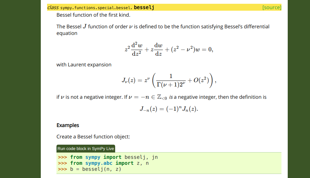
(from https://docs.sympy.org/dev/modules/functions/special.html#sympy.functions.special.bessel.besselj)
However, the source for this math in the docstring of the function uses RST syntax:
class besselj(BesselBase):
    """
    Bessel function of the first kind.

    The Bessel `J` function of order `\nu` is defined to be the function
    satisfying Bessel's differential equation

    .. math ::
        z^2 \frac{\mathrm{d}^2 w}{\mathrm{d}z^2}
        + z \frac{\mathrm{d}w}{\mathrm{d}z} + (z^2 - \nu^2) w = 0,

    with Laurent expansion

    .. math ::
        J_\nu(z) = z^\nu \left(\frac{1}{\Gamma(\nu + 1) 2^\nu} + O(z^2) \right),

    if :math:`\nu` is not a negative integer. If :math:`\nu=-n \in \mathbb{Z}_{<0}`
    *is* a negative integer, then the definition is

    .. math ::
        J_{-n}(z) = (-1)^n J_n(z).
Furthermore, in SymPy's documentation we have configured it so that text
between `single backticks` is rendered as math. This was originally done for
convenience, as the alternative way is to write :math:`\nu` every
time you want to use inline math. But this has lead to many people being
confused, as they are used to Markdown where `single backticks` produce
code.
A better way to write this would be if we could delimit math with dollar
signs, like $\nu$. This is how things are done in LaTeX documents, as well
as in things like the Jupyter notebook.
With the new sphinx-math-dollar
Sphinx extension, this is now possible. Writing $\nu$ produces $\nu$, and
the above docstring can now be written as
class besselj(BesselBase):
    """
    Bessel function of the first kind.

    The Bessel $J$ function of order $\nu$ is defined to be the function
    satisfying Bessel's differential equation

    .. math ::
        z^2 \frac{\mathrm{d}^2 w}{\mathrm{d}z^2}
        + z \frac{\mathrm{d}w}{\mathrm{d}z} + (z^2 - \nu^2) w = 0,

    with Laurent expansion

    .. math ::
        J_\nu(z) = z^\nu \left(\frac{1}{\Gamma(\nu + 1) 2^\nu} + O(z^2) \right),

    if $\nu$ is not a negative integer. If $\nu=-n \in \mathbb{Z}_{<0}$
    *is* a negative integer, then the definition is

    .. math ::
        J_{-n}(z) = (-1)^n J_n(z).
We also plan to add support for $$double dollars$$ for display math so that .. math :: is no longer needed either .
For end users, the documentation on docs.sympy.org will continue to render exactly the same, but for developers, it is much easier to read and write.
This extension can be easily used in any Sphinx project. Simply install it with pip or conda:
pip install sphinx-math-dollar
or
conda install -c conda-forge sphinx-math-dollar
Then enable it in your conf.py:
extensions = ['sphinx_math_dollar', 'sphinx.ext.mathjax']
Google Season of Docs
The above work on sphinx-math-dollar is part of work I have been doing to improve the tooling around SymPy's documentation. This has been to assist our technical writer Lauren Glattly, who is working with SymPy for the next three months as part of the new Google Season of Docs program. Lauren's project is to improve the consistency of our docstrings in SymPy. She has already identified many key ways our docstring documentation can be improved, and is currently working on a style guide for writing docstrings. Some of the issues that Lauren has identified require improved tooling around the way the HTML documentation is built to fix. So some other SymPy developers and I have been working on improving this, so that she can focus on the technical writing aspects of our documentation.
Lauren has created a draft style guide for documentation at https://github.com/sympy/sympy/wiki/SymPy-Documentation-Style-Guide. Please take a moment to look at it and if you have any feedback on it, comment below or write to the SymPy mailing list.
August 23, 2019

|
|
“Software is like entropy: It is difficult to grasp, weighs nothing, and obeys the Second Law of Thermodynamics; i.e., it always increases.” — Norman Augustine Welcome everyone, this is your host Nikhil Maan aka Sc0rpi0n101 and this week will be the last week of coding for GSoC 2019. It is time to finish work now. The C Parser Travis Build Tests Documentation The C Parser I completed the C Parser last week along with the documentation for the module.
August 22, 2019
|
|
|
Welcome everyone, this is your host Nikhil Maan aka Sc0rpi0n101 and this week we’re talking about the C parser. The Fortran Parser The C Parser Documentation Travis Build The Fortran Parser The Fortran Parser is complete. The Pull Request has also been merged. The parser is merged in master and will be a part of the next SymPy release. You can check out the source code for the Parser at the Pull Request.
August 20, 2019

|
|
The last week of coding period is officially over. A summary of the work done during this week is:
- #17379 is now complete and currently under review. I will try to get it merged within this week.
- #17392 still needs work. I will try to put a closure to this by the end of week.
- #17440 was started. It attempts to add a powerful (but optional) SAT solving engine to SymPy (pycosat). The performance gain for SAT solver is also subtle here: Using this
1
2
3
4
from sympy import *
from sympy.abc import x
r = random_poly(x, 100, -100, 100)
ans = ask(Q.positive(r), Q.positive(x))
The performance is like
1
2
3
4
5
6
7
8
# In master
 |  `- 0.631 check_satisfiability  sympy/assumptions/satask.py:30
 |     `- 0.607 satisfiable  sympy/logic/inference.py:38
 |        `- 0.607 dpll_satisfiable  sympy/logic/algorithms/dpll2.py:21
# With pycosat
 |  `- 0.122 check_satisfiability  sympy/assumptions/satask.py:30
 |     `- 0.098 satisfiable  sympy/logic/inference.py:39
 |        `- 0.096 pycosat_satisfiable  sympy/logic/algorithms/pycosat_wrapper.py:11
It is finished and under review now.
Also, with the end of GSoC 2019, final evaluations have started. I will be writing a final report to the whole project by the end of this week.
So far it has been a great and enriching experience for me. It was my first attempt at GSoC and I am lucky to get such an exposure. I acknowledge that I started with an abstract idea of the project but I now understand both the need and the code of New Assumptions pretty well (thanks to Aaron who wrote the most of it). The system is still in its early phases and needs a lot more work. I am happy to be a part of it and I will be available to work on it.
This is the last weekly report but I will still be contributing to SymPy and open source in general. I will try to write more of such experiences through this portal. Till then, Good bye and thank you!
|
|
|
This was the last week of the coding period. With not much of work left, the goal was to wrap-up the PR’s.
The week started with the merge of PR #17001 which implemented a method cut_section() in the polygon class, in order to get two new polygons when a polygon is cut via a line. After this a new method first_moment_of_area() was added in PR #17153. This method used cut_section() for its implementation. Tests for the same were added in this PR. Also the existing documentation was improved. I also renamed the polar_modulus() function to polar_second_moment_of_area() which was a more general term as compared to the previous name. This PR also got merged later on.
Now, we are left with two more PR’s to go. PR #17122 (Column Buckling) and PR #17345 (Beam diagram). The column buckling probably requires a little more documentation. I will surely look into it and add some more explanations and references to it. Also, the beam diagram PR has been completed and documented. A few more discussions to be done on its working and we will be ready with it.
I believe that by the end of this week both of these will finally get a merge.
Another task that remains is the implementation of the Truss class. Some rigorous debate and discussion is still needed to be done before we start its implementation. Once we agree on the implementation needs and API it won’t be a difficult task to write it through.
Also, since the final evaluations have started I will be writing the project report which I have to submit before the next week ends.
Since officially the coding period ends here, there would be no ToDo’s for the next week, just the final wrapping up and will surely try to complete the work that is still left.
Will keep you updated!
Thanks!

|
|
Week 12 ends.. - So, finally after a long summer GSoC has come to an end!! It has been a great experience, and something which I will cherish for the rest of my life. I would like to thank my mentor Sartaj, who has been guiding me through the thick and thin of times....
August 19, 2019

|
|
We’ve reached to the end of GSoC 2019, end to the really productive and wonderful summer. In the last two weeks I worked on documenting polycyclic groups which got merged as well, here is the PR sympy/sympy#17399.
Also, the PR on Induced-pcgs and exponent vector for polycyclic subgroups got merged sympy/sympy#17317.
Let’s have a look at some of the highlights of documentation.
- The parameters of both the classes(
PolycyclicGroupandCollector) has been discussed in detail. - Conditions for a word to be collected or uncollected is highlighted.
- Computation of polycyclic presentation has been explained in detail highlighting the sequence in which presentation is computed with the corresponding pcgs and and polycyclic series elements used.
- Other methods like
subword_index,exponent_vector,depth, etc are also documented.
An example is provided for every functionality. For more details one can visit: https://docs.sympy.org/dev/modules/combinatorics/pc_groups.html
Now, I’m supposed to prepare a final report presenting all the work done. Will update with report next week.
In addition to the report preparation I’ll try to add Parameters section in the docstrings for various classes and methods of pc_groups.
August 18, 2019

|
|
It’s finally the last week of the Google Summer of Code 2019. Before I start discussing my work over the summer I would like to highlight my general experience with the GSoC program.
GSoC gives students all over the world the opportunity to connect and collaborate with some of the best programmers involved in open source from around the world. I found the programme tremendusly enriching both in terms of the depth in which I got to explore some of the areas involved in my project and also gave me exxposure to some areas I had no previous idea about. The role of a mentor in GSoC is the most important and I consider myself very lucky to have got Yathartha Anirudh Joshi and Amit Kumar as my mentors. Amit and Yathartha has been tremendously encouraging and helpful throughout the summer. I would also like to mention the importance of the entire community involved, just being part of the SymPy community.
Work Completed
Here is a list of PRs which were opened during the span of GSoC:
-
#16796 Added
_solve_modularfor handling equations a - Mod(b, c) = 0 where only b is expr -
#16890 Fixing lambert in bivariate to give all real solutions
-
#17043 Feature power_list to return all powers of a variable present in f
Here is a list of PRs merged:
-
#16796 Added
_solve_modularfor handling equations a - Mod(b, c) = 0 where only b is expr -
#16890 Fixing lambert in bivariate to give all real solutions
Here is all the brief description about the PRs merged:
In this PR a new solver _solve_modular was made for solving modular equations.
What type of equations to be considered and what domain?
A - Mod(B, C) = 0

    A -> This can or cannot be a function specifically(Linear, nth degree single
         Pow, a**f_x and Add and Mul) of symbol.(But currently its not a
        function of x)
    B -> This is surely a function of symbol.
    C -> It is an integer.
And domain should be a subset of S.Integers.
Filtering out equations
A check is being applied named _is_modular which verifies that only above
mentioned type equation should return True.
Working of _solve_modular
In the starting of it there is a check if domain is a subset of Integers.
domain.is_subset(S.Integers)
Only domain of integers and it subset are being considered while solving these equations. Now after this it separates out a modterm and the rest term on either sides by this code.
modterm = list(f.atoms(Mod))[0]
rhs = -(S.One)*(f.subs(modterm, S.Zero))
if f.as_coefficients_dict()[modterm].is_negative:
    # f.as_coefficient(modterm) was returning None don't know why
    # checks if coefficient of modterm is negative in main equation.
    rhs *= -(S.One)
Now the equation is being inverted with the helper routine _invert_modular
like this.
n = Dummy('n', integer=True)
f_x, g_n = _invert_modular(modterm, rhs, n, symbol)
I am defining n in _solve_modular because _invert_modular contains
recursive calls to itself so if define the n there then it was going to have
many instances which of no use. Thats y I am defining it in _solve_modular.
Now after the equation is inverted now solution finding takes place.
if f_x is modterm and g_n is rhs:
        return unsolved_result
First of all if _invert_modular fails to invert then a ConditionSet is being
returned.
    if f_x is symbol:
        if domain is not S.Integers:
            return domain.intersect(g_n)
        return g_n
And if _invert_modular is fully able to invert the equation then only domain
intersection needs to takes place. _invert_modular inverts the equation
considering S.Integers as its default domain.
    if isinstance(g_n, ImageSet):
        lamda_expr = g_n.lamda.expr
        lamda_vars = g_n.lamda.variables
        base_set = g_n.base_set
        sol_set = _solveset(f_x - lamda_expr, symbol, S.Integers)
        if isinstance(sol_set, FiniteSet):
            tmp_sol = EmptySet()
            for sol in sol_set:
                tmp_sol += ImageSet(Lambda(lamda_vars, sol), base_set)
            sol_set = tmp_sol
        return domain.intersect(sol_set)
In this case when g_n is an ImageSet of n and f_x is not symbol so the
equation is being solved by calling _solveset (this will not lead to
recursion because equation to be entered is free from Mod) and then
the domain intersection takes place.
What does _invert_modular do?
This function helps to convert the equation A - Mod(B, C) = 0 to a
form (f_x, g_n).
First of all it checks the possible instances of invertible cases if not then
it returns the equation as it is.
a, m = modterm.args
if not isinstance(a, (Dummy, Symbol, Add, Mul, Pow)):
        return modterm, rhs
Now here is the check for complex arguments and returns the equation as it is if somewhere it finds I.
if rhs.is_real is False or any(term.is_real is False \
            for term in list(_term_factors(a))):
        # Check for complex arguments
        return modterm, rhs
Now after this we check of emptyset as a solution by checking range of both sides of equation. As modterm can have values between [0, m - 1] and if rhs is out of this range then emptySet is being returned.
if (abs(rhs) - abs(m)).is_positive or (abs(rhs) - abs(m)) is S.Zero:
        # if rhs has value greater than value of m.
        return symbol, EmptySet()
Now the equation haveing these types are being returned as the following
if a is symbol:
        return symbol, ImageSet(Lambda(n, m*n + rhs), S.Integers)

    if a.is_Add:
        # g + h = a
        g, h = a.as_independent(symbol)
        if g is not S.Zero:
            return _invert_modular(Mod(h, m), (rhs - Mod(g, m)) % m, n, symbol)

    if a.is_Mul:
        # g*h = a
        g, h = a.as_independent(symbol)
        if g is not S.One:
            return _invert_modular(Mod(h, m), (rhs*invert(g, m)) % m, n, symbol)
The more peculiar case is of a.is_Pow which is handled as following.
if a.is_Pow:
        # base**expo = a
        base, expo = a.args
        if expo.has(symbol) and not base.has(symbol):
            # remainder -> solution independent of n of equation.
            # m, rhs are made coprime by dividing igcd(m, rhs)
            try:
                remainder = discrete_log(m / igcd(m, rhs), rhs, a.base)
            except ValueError: # log does not exist
                return modterm, rhs
            # period -> coefficient of n in the solution and also referred as
            # the least period of expo in which it is repeats itself.
            # (a**(totient(m)) - 1) divides m. Here is link of theoram:
            # (https://en.wikipedia.org/wiki/Euler's_theorem)
            period = totient(m)
            for p in divisors(period):
                # there might a lesser period exist than totient(m).
                if pow(a.base, p, m / igcd(m, a.base)) == 1:
                    period = p
                    break
            return expo, ImageSet(Lambda(n, period*n + remainder), S.Naturals0)
        elif base.has(symbol) and not expo.has(symbol):
            remainder_list = nthroot_mod(rhs, expo, m, all_roots=True)
            if remainder_list is None:
                return symbol, EmptySet()
            g_n = EmptySet()
            for rem in remainder_list:
                g_n += ImageSet(Lambda(n, m*n + rem), S.Integers)
            return base, g_n
Two cases are being created based of a.is_Pow
- x**a
- a**x
x**a - It is being handled by the helper function nthroot_mod which returns
required solution. I am not going into very mch detail for more
information you can read the documentation of nthroot_mod.
a**x - For this totient is being used in the picture whose meaning can be
find on this Wikipedia
page. And then its divisors are being checked to find the least period
of solutions.
This PR went through many up and downs and nearly made to the most commented PR. And with the help of @smichr it was successfully merged. It mainly solved the bug for not returning all solutions of lambert.
Explaining the function _solve_lambert (main function to solve lambert equations)
Input - f, symbol, gens
OutPut - Solution of f = 0 if its lambert type expression else NotImplementedError
This function separates out cases as below based on the main function present in the main equation.
For the first ones:
1a1) B**B = R != 0 (when 0, there is only a solution if the base is 0,
                   but if it is, the exp is 0 and 0**0=1
                   comes back as B*log(B) = log(R)
1a2) B*(a + b*log(B))**p = R or with monomial expanded or with whole
                            thing expanded comes back unchanged
   log(B) + p*log(a + b*log(B)) = log(R)
   lhs is Mul:
       expand log of both sides to give:
       log(B) + log(log(B)) = log(log(R))
1b) d*log(a*B + b) + c*B = R
   lhs is Add:
       isolate c*B and expand log of both sides:
       log(c) + log(B) = log(R - d*log(a*B + b))
If the equation are of type 1a1, 1a2 and 1b then the mainlog of the equation is taken into concern as the deciding factor lies in the main logarithmic term of equation.
For the next two,
   collect on main exp
   2a) (b*B + c)*exp(d*B + g) = R
       lhs is mul:
           log to give
           log(b*B + c) + d*B = log(R) - g
   2b) -b*B + g*exp(d*B + h) = R
       lhs is add:
           add b*B
           log and rearrange
           log(R + b*B) - d*B = log(g) + h
If the equation are of type 2a and 2b then the mainexp of the equation is taken into concern as the deciding factor lies in the main exponential term of equation.
3) d*p**(a*B + b) + c*B = R
   collect on main pow
   log(R - c*B) - a*B*log(p) = log(d) + b*log(p)
If the equation are of type 3 then the mainpow of the equation is taken into concern as the deciding factor lies in the main power term of equation.
Eventually from all of the three cases the equation is meant to be converted to this form:-
f(x, a..f) = a*log(b*X + c) + d*X - f = 0 which has the
solution,  X = -c/b + (a/d)*W(d/(a*b)*exp(c*d/a/b)*exp(f/a)).
And the solution calculation process is done by _lambert function.
Everything seems flawless?? You might be thinking no modification is required. Lets see what loopholes are there in it.
What does PR #16890 do?
There are basically two flaws present with the this approach.
- Not considering all branches of equation while taking log both sides.
- Calculation of roots should consider all roots in case having rational power.
1. Not considering all branches of equation while taking log both sides.
Let us consider this equation to be solved by _solve_lambert function.
-1/x**2 + exp(x/2)/2 = 0
So what the old _solve_lambert do is to convert this equation to following.
2*log(x) + x/2 = 0
and calculates its roots from _lambert.
But it missed this branch of equation while taking log on main equation.
2*log(-x) + x/2 = 0
Yeah you can reproduce the original equation from this equation.So basically the problem was that it missed the branches of equation while taking log. And when does the main equation have more than one branch?? The terms having even powers of variable x leads to two different branches of equation.
So how it is solved?
What I has done is that before actually gets into solving I preprocess the main equation
and if it has more than one branches of equation while converting taking log then I consider
all the equations generated from them.(with the help of _solve_even_degree_expr)
How I preprocess the equation? So what I do is I replace all the even powers of x present with even powers of t(dummy variable).
Code for targeted replacement
lhs = lhs.replace(
            lambda i:  # find symbol**even
                i.is_Pow and i.base == symbol and i.exp.is_even,
            lambda i:  # replace t**even
                t**i.exp)
Example:-
Main equation -> -1/x**2 + exp(x/2)/2 = 0
After replacement -> -1/t**2 + exp(x/2)/2 = 0
Now I take logarithms on both sides and simplify it.
After simplifying -> 2*log(t) + x/2 = 0
Now I call function _solve_even_degree_expr to replace the t with +/-x to generate two equations.
Replacing t with +/-x
1. 2*log(x) + x/2 = 0
2. 2*log(-x) + x/2 = 0
And consider the solutions of both of the equations to return all lambert real solutions
of -1/x**2 + exp(x/2)/2 = 0.
Hope you could understand the logic behind this work.
2. Calculation of roots should consider all roots in case having rational power.
This flaw is in the calculation of roots in function _lambert.
Earlier the function_lambert has the working like :-
- Find all the values of a, b, c, d, e in the required loagrithmic equation
- Then it defines a solution of the form
-c/b + (a/d)*l where l = LambertW(d/(a*b)*exp(c*d/a/b)*exp(-f/a), k)and then it included that solution. I agree everything seems flawless here. but try to see the step where we are defining l.
Let us suppose a hypothetical algorithm just like algorithm used in _lambert
in which equation to be solved is
x**3 - 1 = 0
and in which we define solution of the form
x = exp(I*2*pi/n) where n is the power of x in equation
so the algorithm will give solution
x = exp(I*2*pi/3) # but expected was [1, exp(I*2*pi/3), exp(-I*2*pi/3)]
which can be found by finding all solutions of
x**n - exp(2*I*pi) = 0
by a different correct algorithm. Thats y it was wrong.
The above algorithm would have given correct values for x - 1 = 0.
And the question in your mind may arise that why only exp() because the
possiblity of having more than one roots is in exp(), because if the algorithm
would have been like x = a, where a is some real constant then there is not
any possiblity of further roots rather than solution like x = a**(1/n).
And its been done in code like this:
code
num, den = ((c*d-b*f)/a/b).as_numer_denom()
p, den = den.as_coeff_Mul()
e = exp(num/den)
t = Dummy('t')
args = [d/(a*b)*t for t in roots(t**p - e, t).keys()]
Work under development
This PR tends to define a unifying algorithm for linear relations.
Future Work
Here is a list that comprises of all the ideas (which were a part of my GSoC Proposal and/or thought over during the SoC) which can extend my GSoC project.
-
Integrating helper solvers within solveset: linsolve, solve_decomposition, nonlinsolve
-
Handle nested trigonometric equations.
August 13, 2019
|
|
|
With the end of this week the draw() function has been completely implemented. The work on PR #17345 has been completed along with the documentations.
As mentioned in the previous blog this PR was an attempt to make the draw() function use SymPy’s own plot() rather than importing matplotlib externally to plot the diagram. The idea was to plot the load equation which is in terms of singularity function. This would directly plot uniformly distributed load, uniformly varying load and other higher order loads except for point loads and moment loads.
The task was now to plot the remaining parts of the diagram which were:
- A rectangle for drawing the beam
- Arrows for point loads
- Markers for moment loads and supports
- Colour filling to fill colour in inside the higher order loads (order >=0).
Instead of making temporary hacks to implement these, I went a step further to give the plotting module some additional functionalities. Apart from helping in implementing the draw() function, this would also enhance the plotting module.
The basic idea was to have some additional keyworded arguments in the plot() function. Every keyworded argument would be a list of dictionaries where each dictionary would represent the arguments (or parameters) that would have been passed in the corresponding matplotlib functions.
These are the functions of matplotlib that can now be accessed using sympy’s plot(), along with where there are used in our current situation:
- matplotlib.patches.Rectangle -to draw the beam
- matplotlib.pyplot.annotate – to draw arrows of load
- matplotlib.markers– to draw supports and moment loads
- fill_between() – to fill an area with color
Another thing which is worth mentioning is that to use fill_between() we would require numpy’s arange() for sure. Although it might be better if we could avoid using an external module directly, but I guess this is unavoidable for now.
Also, I have added an option for the user to scale the plot and get a pictorial view of it in case where the plotting with the exact dimensions doesn’t produce a decent diagram. For eg. If the magnitude of the load (order >= 0) is relatively higher to other applied loads or to the length of the beam, the load plot might get out of the final plot window.
Here is an example:
>>> R1, R2 = symbols('R1, R2')
>>> E, I = symbols('E, I')

>>> b1 = Beam(50, 20, 30)

>>> b1.apply_load(10, 2, -1)
>>> b1.apply_load(R1, 10, -1)
>>> b1.apply_load(R2, 30, -1)
>>> b1.apply_load(90, 5, 0, 23)
>>> b1.apply_load(10, 30, 1, 50)
>>> b1.apply_support(50, "pin")
>>> b1.apply_support(0, "fixed")
>>> b1.apply_support(20, "roller")
# case 1 on the left
>>> p = b1.draw()
>>> p.show()

# case 2 on the right
>>> p1 = b1.draw(pictorial=True)
>>> p1.show()

Next Week:
- Getting leftover PR’s merged
- Initiating implementation of Truss class
Will keep you updated!
Thanks!
August 12, 2019
|
|
|
So, the second last week of the official coding period is over now. During the last two weeks, I was mostly occupied with on-campus placement drives, hence I couldn’t put up a blog earlier. A summary of my work during these weeks is as follows:
-
First of all, #17144 is merged 😄. This was a large PR and hence took time to get fully reviewed. With this, the performance of New assumptions comes closer to that of the old system. Currently, queries are evaluated about 20X faster than before.
- #17379 attempts to remove SymPy’s costly rcall() from the whole assumptions mechanism. It’s a follow-up from #17144 and the performance gain is subtle for large queries. E.g.
1
2
3
from sympy import *
p = random_poly(x, 50, -50, 50)
print(ask(Q.positive(p), Q.positive(x)))
In the master it takes
4.292 s, out of this2.483 sis spent in rcall. With this, the time spent is1.929 sand0.539 srespectively. - #17392 attempts to make the New Assumptions able to handle queries which involve Relationals. Currently, it works only with simple queries (e.g.
ask(x>y, Q.positive(x) & Q.negative(y))now evaluatesTrue) just like the way old system works. This is a much-awaited functionality for the new system. Also, during this I realized that sathandlers lack many necessary facts. This PR also adds many new facts to the system.
For the last week of coding, my attempt would be to complete both of these PRs and get them merged. Also, I will try to add new facts to sathandlers.
|
|
|
Week 11 ends.. - The second last week has also come to an end. We are almost there at the end of the ride. Me and Sartaj had a meeting on 13th of August about the final leftovers to be done, and wrapping up the GSoC work successfully. Here are the works which have...
August 11, 2019
This was the eleventh week meeting with the GSoC mentors which was scheduled on
Sunday 11th August, 2019 between 11:30 - 12:30 PM (IST). Me, Yathartha and Amit
were the attendees of the meeting. _solve_modular was discussed in this meeting.
Here is all the brief description about new solver _solve_modular for solving
modular equations.
What type of equations to be considered and what domain?
A - Mod(B, C) = 0

    A -> This can or cannot be a function specifically(Linear, nth degree single
         Pow, a**f_x and Add and Mul) of symbol.(But currently its not a
        function of x)
    B -> This is surely a function of symbol.
    C -> It is an integer.
And domain should be a subset of S.Integers.
Filtering out equations
A check is being applied named _is_modular which verifies that only above
mentioned type equation should return True.
Working of _solve_modular
In the starting of it there is a check if domain is a subset of Integers.
domain.is_subset(S.Integers)
Only domain of integers and it subset are being considered while solving these equations. Now after this it separates out a modterm and the rest term on either sides by this code.
modterm = list(f.atoms(Mod))[0]
rhs = -(S.One)*(f.subs(modterm, S.Zero))
if f.as_coefficients_dict()[modterm].is_negative:
    # f.as_coefficient(modterm) was returning None don't know why
    # checks if coefficient of modterm is negative in main equation.
    rhs *= -(S.One)
Now the equation is being inverted with the helper routine _invert_modular
like this.
n = Dummy('n', integer=True)
f_x, g_n = _invert_modular(modterm, rhs, n, symbol)
I am defining n in _solve_modular because _invert_modular contains
recursive calls to itself so if define the n there then it was going to have
many instances which of no use. Thats y I am defining it in _solve_modular.
Now after the equation is inverted now solution finding takes place.
if f_x is modterm and g_n is rhs:
        return unsolved_result
First of all if _invert_modular fails to invert then a ConditionSet is being
returned.
    if f_x is symbol:
        if domain is not S.Integers:
            return domain.intersect(g_n)
        return g_n
And if _invert_modular is fully able to invert the equation then only domain
intersection needs to takes place. _invert_modular inverts the equation
considering S.Integers as its default domain.
    if isinstance(g_n, ImageSet):
        lamda_expr = g_n.lamda.expr
        lamda_vars = g_n.lamda.variables
        base_set = g_n.base_set
        sol_set = _solveset(f_x - lamda_expr, symbol, S.Integers)
        if isinstance(sol_set, FiniteSet):
            tmp_sol = EmptySet()
            for sol in sol_set:
                tmp_sol += ImageSet(Lambda(lamda_vars, sol), base_set)
            sol_set = tmp_sol
        return domain.intersect(sol_set)
In this case when g_n is an ImageSet of n and f_x is not symbol so the
equation is being solved by calling _solveset (this will not lead to
recursion because equation to be entered is free from Mod) and then
the domain intersection takes place.
What does _invert_modular do?
This function helps to convert the equation A - Mod(B, C) = 0 to a
form (f_x, g_n).
First of all it checks the possible instances of invertible cases if not then
it returns the equation as it is.
a, m = modterm.args
if not isinstance(a, (Dummy, Symbol, Add, Mul, Pow)):
        return modterm, rhs
Now here is the check for complex arguments and returns the equation as it is if somewhere it finds I.
if rhs.is_real is False or any(term.is_real is False \
            for term in list(_term_factors(a))):
        # Check for complex arguments
        return modterm, rhs
Now after this we check of emptyset as a solution by checking range of both sides of equation. As modterm can have values between [0, m - 1] and if rhs is out of this range then emptySet is being returned.
if (abs(rhs) - abs(m)).is_positive or (abs(rhs) - abs(m)) is S.Zero:
        # if rhs has value greater than value of m.
        return symbol, EmptySet()
Now the equation haveing these types are being returned as the following
if a is symbol:
        return symbol, ImageSet(Lambda(n, m*n + rhs), S.Integers)

    if a.is_Add:
        # g + h = a
        g, h = a.as_independent(symbol)
        if g is not S.Zero:
            return _invert_modular(Mod(h, m), (rhs - Mod(g, m)) % m, n, symbol)

    if a.is_Mul:
        # g*h = a
        g, h = a.as_independent(symbol)
        if g is not S.One:
            return _invert_modular(Mod(h, m), (rhs*invert(g, m)) % m, n, symbol)
The more peculiar case is of a.is_Pow which is handled as following.
if a.is_Pow:
        # base**expo = a
        base, expo = a.args
        if expo.has(symbol) and not base.has(symbol):
            # remainder -> solution independent of n of equation.
            # m, rhs are made coprime by dividing igcd(m, rhs)
            try:
                remainder = discrete_log(m / igcd(m, rhs), rhs, a.base)
            except ValueError: # log does not exist
                return modterm, rhs
            # period -> coefficient of n in the solution and also referred as
            # the least period of expo in which it is repeats itself.
            # (a**(totient(m)) - 1) divides m. Here is link of theoram:
            # (https://en.wikipedia.org/wiki/Euler's_theorem)
            period = totient(m)
            for p in divisors(period):
                # there might a lesser period exist than totient(m).
                if pow(a.base, p, m / igcd(m, a.base)) == 1:
                    period = p
                    break
            return expo, ImageSet(Lambda(n, period*n + remainder), S.Naturals0)
        elif base.has(symbol) and not expo.has(symbol):
            remainder_list = nthroot_mod(rhs, expo, m, all_roots=True)
            if remainder_list is None:
                return symbol, EmptySet()
            g_n = EmptySet()
            for rem in remainder_list:
                g_n += ImageSet(Lambda(n, m*n + rem), S.Integers)
            return base, g_n
Two cases are being created based of a.is_Pow
- x**a
- a**x
x**a - It is being handled by the helper function nthroot_mod which returns
required solution. I am not going into very mch detail for more
information you can read the documentation of nthroot_mod.
a**x - For this totient is being used in the picture whose meaning can be
find on this Wikipedia
page. And then its divisors are being checked to find the least period
of solutions.
Hope I am able to clear out everything!!
Code improvement takes time!!
August 06, 2019

|
|
For this week, I’ve made some more minor changes to the Indexed pull request from last week, in addition to filing a new matrix wildcard pull request.
Matrix Wildcards (again)
Since #17223 was merged this week, I started with an implementation of matrix wildcards that takes advantage of the functionality included in the pull request. I thought that this would be relatively straightforward, with an implementation of the matches method for the MatrixWild subclass being enough. There was one problem though: the underlying matching implementation assumes that all powers in the expression are an instance of the Pow class. However, this isn’t true for matrix expressions: the MatPow class, which represents matrix powers, is a subclass of its own. I’m not exactly sure what the reason for this is, since a quick change of MatPow to inherit from Pow doesn’t seem to break anything. I’ll probably look into this a bit more, since I think this might have something to do with the fact that Matrix exponents can also include other matrices.
My solution for this was to allow temporarily allow expansion of powers by recursing through the expression tree and setting the is_Pow field of each matrix power to True and later reverting these states later. It doesn’t look pretty, but it does seem to work (you can see the code here).
Next Steps
I’ll try to get started with some optimizations that utilize this wildcard class once the pull request gets merged.
|
|
|
“Software is like entropy: It is difficult to grasp, weighs nothing, and obeys the Second Law of Thermodynamics; i.e., it always increases.” — Norman Augustine Welcome everyone, this is your host Nikhil Maan aka Sc0rpi0n101 and we will talk all about the Fortran Parser this week. I have passed the second evaluation and Fortran Parser pull request is complete. The Week Fortran Parser SymPy Expression Travis Builds The C Parser The Meeting The Week This week began with me working on the C parser to finalize that.
August 05, 2019
|
|
|
This was the end of the tenth week, and we have entered the final phase of the project.
For the last phase we have Truss calculations to be implemented in the continuum_mechanics module. I had initiated a discussion regarding what needs to be done and how the implementation will move forward in an issue #17302. We will have to analyse a bit more about making Truss calculations symbolic and what benefits one might get in solving it symbolically. We have some good packages to compare from like this. I guess a bit more discussion is needed before we go ahead with it.
Besides this, I had worked on improving the draw() function implemented in the previous week in PR #17240. I modified it to use the _backend attribute for plotting the beam diagram. This could have worked until I realised that using the _backend attribute doesn’t really has affect the Plot object. To understand the last statement, lets go to how sympy.plot() works.
In simple terms, the equations that we pass through the plot() function as arguments are actually stored in _series attribute. So we can indirectly say that the basic data of the plot is stored in this attribute. But using the _backend attribute wouldn’t alter _series at all and if _series remains empty at the start it would end up storing nothing.
But we are of course getting a decent plot at the end, so shouldn’t we probably ignore this? No, it would surely give the plot but we won’t be getting a fully defined Plot object which we can further use with PlotGrid to get a subplot which includes all the five plots related to the beam.
Keeping this in mind, I tried an alternative way to directly use sympy.plot() to give the plot. Although a bit hard and time taking to do, I have intiated this in a draft PR #17345. This PR perfectly plots a rectangular beam and loads (except point and moment loads). Only things that are left here are to plot supports and arrows denoting the direction of the load.
The example below shows how it functions: (keep in mind it just plots the basic structure of the intended beam diagram, it hasn’t been completed yet)
>>> E, I = symbols('E, I')
>>> b = Beam(9, E, I)
>>> b.apply_load(-12, 9, -1)  # gets skipped
>>> b.apply_load(50, 5, -2)  # gets skipped
>>> b.apply_load(3, 6, 1, end=8)
>>> b.apply_load(4, 0, 0, end=5)
>>> b.draw()

I also tried to complete the leftover PR’s in this week, but still some work is left.
Next week:
- Completing the draw() function
- Documentation and testing
- Starting Truss implementations
Will keep you updated!
Thanks!
|
|
|
Week 10 ends.. - Phase 3 of the GSoC coding period is traversong smoothly. !! I and Sartaj had a meeting on the 05th of August, about the timeline of the next 2 weeks. Here are the deliverables that have been completed in this week, including the minutes of the meeting. The second aseries...
|
|
|
The tenth week of coding period has ended and a new PRsympy/sympy#17317 has been introduced. The PR implements induced Pcgs and exponent vector for polycyclic subgroups with respect to the original pcgs of the group. Below is an example to show the functionality.
>>> from sympy.combinatorics import *
>>> S = SymmetricGroup(8)
>>> G = S.sylow_subgroup(2)
>>> gens = [G[0], G[1]]
>>> PcGroup = G.polycyclic_group()
>>> collector = PcGroup.collector
>>> ipcgs = collector.induced_pcgs(gens)
>>> [gen.order() for gen in ipcgs]
[2, 2, 2]
Further it can also be used to implement Canonical polycyclic sequence which can be used to check if two subgroups of polycyclic presented group G are equal or not.
For the next week I’ll try to complete the documentation work on polycyclic groups and open a PR for the same.
Till then, good byee..
August 04, 2019
This was the tenth week meeting with the GSoC mentors which was scheduled on Sunday 4th August, 2019 between 1:00 - 2:00 PM (IST). Me, Yathartha were the attendees of the meeting.
- Discussing previous week’s progress
-
Progress of
_solve_modular:- In PR #16976 After discussing with Yathartha, I decided to change the basic model of the_solve_modularsuch that I should be able to target equations more efficiently and also the rest of the types of equation should return ConditionSet. Cases likeMod(a**x, m) - rhs = 0are special type and will be handled differently with the helper functions of ntheory module. -
Progress of ImageSet Union:- In PR #17079 This PR is currently been left for review.
-
Next week goals
- Work upon
_solve_modular - In the following week I will be changing the domain of solving equations to Integers only.
Code improvement takes time!!
August 01, 2019
|
|
|
Week 9 ends.. - The last phase of this journey has started. I am happy to let you know that I have passed Phase 2 successfully. Phase 3 will include merging of some important code written in Phase 2, and also implementation of some other useful code. I had a meeting with Sartaj in...
July 30, 2019
|
|
|
I spent most of this week getting #17144 ready to be merged. I had to change a lot of things from the last attempt. One of such was an attempt on early encoding, I had tried it on Literals. They were eventually going to be encoded so I tried to do this when Literals were created only. But as Aaron suggested, my approach had left encodings in the global space and hence could leak memory. During the week, I tried to attach encoding to the CNF object itself but it would have needed a lot of refactoring, since CNF objects interacted with other such objects. So, after some attempts, at the end I left the encoding to be done at last in EncodedCNF object. Currently, this is ready to be merged.
For the coming weeks, I would try to improve over this.
This was also the week for second monthly evaluation and I feel happy to announce that I passed it. From this week my college has also started but I am still able to give the required time to this project and complete it.
Will keep you updated. Thank you !
July 29, 2019
|
|
|
With the end of this week the third phase officially ends.
There has been some discussions in the PR #17240 which implements the draw() function. We might change the name of the function to plot() which is more consistent with the previous beam methods plot_shear_force(), plot_bending_moment(), etc.
Another discussion was about making this beam diagram a part of the plot_loading_results(), which basically intends to plot all the beam related plots. Although currently the beam diagram uses matplotlib as an external module, whereas the plot_loading_results() uses PlotGrid which is Sympy’s internal functionality. So it would be a bit tricky to merge those two.
We also discussed the idea or rather the possibility of directly making use of SymPy’s own plot to create a beam diagram. SymPy’s plot() is capable to plotting Singularity functions, so the load applied on the beam can also be plotted using sympy.plot() as beam.load is indeed in terms of singularity function. But there is a problem when it comes to point loads and moment loads as the are in terms singularity function of negative order (or exponent). Not sure whether the sympy plot for singularity functions of negative order is plotted correctly, but the current plot won’t help us in drawing point loads and moment loads. We might have to deal with it separately.
I have opened a discussion in the mailing list regarding whether the plot is correct for singularity functions of negative order, or what else should be done in order to get it corrected.
Also, it will be difficult to plot a rectangle (for making beam) and markers (for making supports) via sympy.plot(). One idea is to go with the _backend attribute of sympy.plot() which helps in directly using the backend (i.e. matplotlib backend). I will have a look over it.
Of course if the beam diagram is made using SymPy’s own plot it would surely be preferred but for that we also need work on sympy.plot() as currently it is limited to certain functionalities.
From the next week I will be starting with the last phase of implementing a Truss structure and its respective calculations.
Since only last few weeks are left, I think I will be able to make a draft PR for the last phase implementation by the end of the next week. And then we would only be left with minor things and leftovers of the previous phases.
Also, I am glad to share that I was able to pass the second evaluations. So once again thank you mentors for all your support and guidance!
Next Week:
- Starting phase-IV implementations
- Simultaneously working and discussing previous PR’s.
Will keep you updated!
Thanks!
|
|
|
Hello everyone, the ninth week of coding period has ended and there is a really good news the polycyclic group PR sympy/sympy#16991 that we were working from the last one and half months is finally merged. This week I didn’t do that much work except organizing different methods and fixing small issues in the above pr to get it merged.
There has been a lot of rearrangement of methods, where most of the methods were moved to the class Collector from the class PolycyclicGroup. Now, we do not need free symbols in-hand, they can be computed by the Collector if not provided by the user. There are few more things which are changed like relative order is computed in the course of polycyclic sequence and series computation. For better look one can go through the above Pr.
I’m hopping to implement few things next week which are mentioned below.
- Induced polycyclic sequence for a subgroup.
- Get started with writing docs for polycyclic groups.
Till then, good byee..
July 28, 2019
|
|
|
Welcome everyone, this is your host Nikhil Maan aka Sc0rpi0n101 and this time we will be talking about the second evaluation for GSoC. The main objective of the week was to get the Fortran parser ready. The Fortran Parser Traivs and the Tests LFortran Evaluation!!! The meeting What Now The Fortran Parser The Fortran parser is finally complete after shifting to using SymPy’s codegen AST. It can now parser all the stuff that the parser could do before shifting.
Planet SymPy is made from the blogs of SymPy's contributors. The opinions it contains are those of the contributor. This site is powered by Rawdog and Rawdog RSS. Feed readers can read Planet SymPy with RSS, FOAF or OPML.